SAT.NET // SENTINEL-2 · MODIS · HANSEN · GHSL · VIIRS · OSM
SYS.OP.NORMAL·2026.09.25 · 16:46:49 UTC
◢ THE SCIENCE BEHIND
Audit-grade measurement, peer-reviewed by design.
EarthVolution does not invent numbers. Every measurement you see on the mission console comes from a published, peer-reviewed dataset — Sentinel-2 imagery from the European Space Agency, the Joint Research Centre of the European Commission, Google Research, and the OpenStreetMap community. This page documents exactly how that pipeline works, what each measurement means, what its expected error is, and where to find the underlying scientific reference for everything.
◢ PLANETARY CASE STUDIES
Three planets, three measured stories.
Real scans from the same Mission Console you use — precomputed against three iconic sites where the satellite record captures a decade of measurable change. Drag the dividers, then open any one live to see all 8 parameters and the AI narrative.
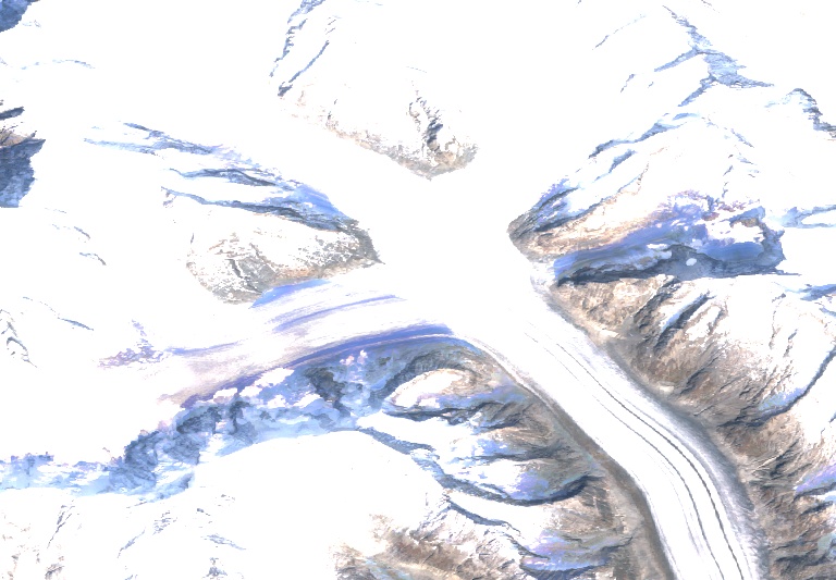
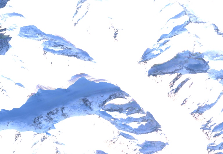
Aletsch Glacier
Valais · Switzerland
46.50°N
8.03°E
◢ 2016 · ARCHIVE
2025 · LIVE ◣
RES 10m/px · S2 L2A
ICE COVER
89,705,943 m² → 75,331,575 m²
-16.0%
The Alps' longest glacier (≈23 km); a UNESCO heritage site. Within this 10 km AOI over the central ice tongue (Konkordiaplatz to Mährjenboden), NASA MODIS MOD10A1 NDSI Snow Cover (Hall et al. 2002) records a 16.0 % drop in persistent snow/ice classification between 2016 and 2025. The retreat tracks the Swiss Federal Office for the Environment's published mass-balance data: Aletsch loses tens of metres of length per year, exposing fresh moraine that the classifier picks up as bare ground.
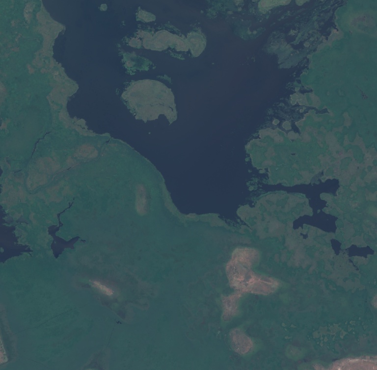
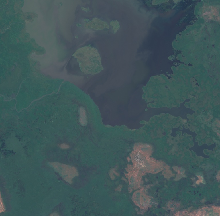
Sahelian endorheic lake — the 1960s extent shrunk by ~90%. This AOI sits on the southern shoreline near the Hadejia-Yobe inflow, where seasonal water extent is most sensitive to upstream rainfall. JRC Global Surface Water (Pekel et al. 2016, Nature) measures a 55.9 % drop in classified surface water between 2016 and 2025. The lake's long-term ~90 % shrinkage (Coe & Foley, JGR 2001) happened mostly in the 1970s–80s; the 2016→25 window captures shoreline oscillation driven by Sahel rainfall variability.
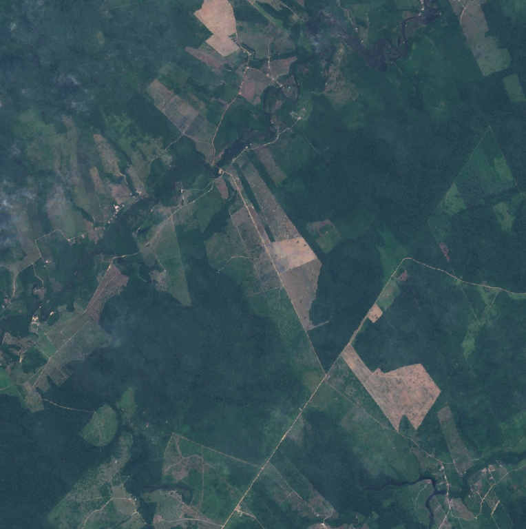
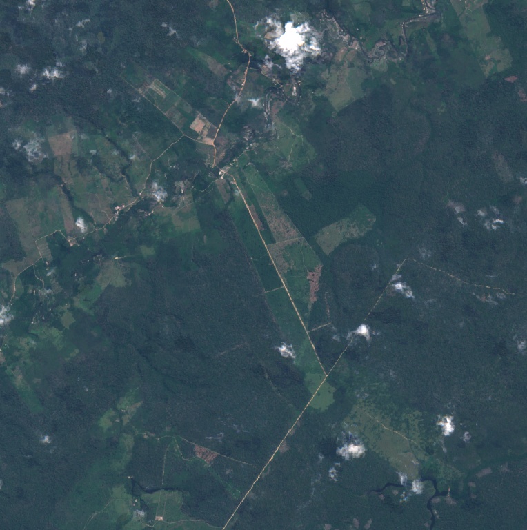
BR-163 / Cuiabá–Santarém highway agricultural expansion zone. Measured against Hansen Global Forest Change v1.13 (Hansen et al. 2013, Science) — the peer-reviewed gold standard the IPCC, FAO and Global Forest Watch cite. Within this 10 km AOI on the BR-163 corridor, 39,647,621 m² of ≥30 %-canopy primary forest was cleared between 2016 and 2024 — a 55.1 % loss. The cleared land is now soy and pasture, both of which Dynamic World still classifies as vegetation; only Hansen's annual loss-year mask catches this conversion.
⚠ Dynamic World V1's clear-sky coverage was sparse over Amazonia in the first half of 2016 (heavy wet-season cloud cover). The imagery baseline was auto-shifted to 2017. The forest-loss metric itself is from Hansen GFC 2016–2024, which is unaffected.
You draw an Area-of-Interest. We pull Sentinel-2 median composites from Google Earth Engine for July–December of 2016 and 2025 — the equalised six-month window eliminates seasonal bias.
STEP 2 · CLASSIFY
Each parameter is measured by its best-in-class peer-reviewed dataset, then cross-validated against an independent satellite or product before the number reaches the screen. Vegetation uses NDVI from Sentinel-2 B8 + B4 (Tucker, 1979), cross-validated against MODIS MOD13Q1 NDVI (Didan, 2015) — when the two satellites agree (Δ < 0.05), confidence is HIGH. EVI (Huete, 2002) is computed in parallel for dense-canopy AOIs where NDVI saturates. Sand uses BSI from Sentinel-2 (Rikimaru, 2002) — a continuous radiometric bare-soil index, immune to the class-boundary wobble of a hard classifier. Water uses JRC Global Surface Water v1.4 + YearlyHistory (Pekel et al., 2016, Nature). Ice & snow use NASA MODIS MOD10A1 NDSI Snow Cover (Hall et al., 2002). Forests use Hansen Global Forest Change v1.13 (Hansen et al., 2013, Science) — closed-canopy only; for tropical AOIs an additional JRC TMF v1 (Vancutsem et al., 2021) layer catches selective logging and degradation that Hansen misses. Buildings use Open Buildings v3 polygons (where covered) plus the multi-temporal JRC GHSL built-up raster for the historical delta. Roads + infrastructure come from OpenStreetMap as a current-state snapshot, with NOAA VIIRS Nighttime Lights (Elvidge et al., 2017) and JRC GHSL Population (Schiavina et al., 2023) jointly providing the 2016 → 2025 human-activity Δ. All Sentinel-2 imagery is cloud-masked at the pixel level via the COPERNICUS/S2_CLOUD_PROBABILITY mask (≥ 40 % probability = masked) and composited on a phenology-matched window (NH summer / SH summer / tropical full-year) so seasonal drift cannot masquerade as change. The number of cloud-free observations that fed each composite is surfaced as the S2 obs · confidence badge beneath every scan.
STEP 3 · INTERPRET
Numbers are written to a deterministic, cached result. A research-mode prompt is sent to Claude Haiku 4.5 with both RGB composites + both land-cover maps + the authoritative pixel counts; it produces a hedged peer-review-style narrative — but is forbidden from inventing or restating numbers.
02 // DATASETS & ACCURACY
Eight measurements, eight peer-reviewed sources
PARAMETER
DATASET
EXPECTED ERROR
CITATION
Water
JRC Global Surface Water + OpenStreetMap
± 5–15 %
Pekel, J.-F. et al. (2016). Nature, 540, 418–422. doi:10.1038/nature20584
Ice / Snow
NASA MODIS MOD10A1 NDSI Snow Cover (NSIDC)
± 5–10 %
Hall, D. K., Riggs, G. A. & Salomonson, V. V. (2002). Remote Sensing of Environment, 83, 181–194. doi:10.1016/S0034-4257(02)00095-0
Vegetation
Sentinel-2 NDVI (Tucker 1979)
± 5 %
Tucker, C. J. (1979). Red and photographic infrared linear combinations for monitoring vegetation. Remote Sensing of Environment, 8(2), 127–150. doi:10.1016/0034-4257(79)90013-0
Forests
Hansen Global Forest Change v1.13 (UMD / Google / USGS)
± 5–10 %
Hansen, M. C. et al. (2013). Science, 342(6160), 850–853. doi:10.1126/science.1244693
Sand / Bare
Sentinel-2 BSI (Rikimaru 2002)
± 5 %
Rikimaru, A., Roy, P. S. & Miyatake, S. (2002). Tropical forest cover density mapping. Tropical Ecology, 43(1), 39–47.
Buildings · count
Google Open Buildings v3 (polygons)
± 5 %
Sirko, W. et al. (2023). arXiv:2107.12283; v3 release: Google Research, 2023.
Buildings · 2016→2025 delta
JRC GHSL Built-up Surface (multi-temporal)
± 10 %
Pesaresi, M., Politis, P. (2023). GHSL Data Package 2023. Joint Research Centre, EU.
Roads
OpenStreetMap (snapshot, way length) + VIIRS Δ
± 5 % OSM · 10 % VIIRS
Haklay, M. (2010). How good is volunteered geographical information? Environment and Planning B, 37(4), 682–703. doi:10.1068/b35097 — Elvidge, C. D. et al. (2017). VIIRS night-time lights. International Journal of Remote Sensing, 38(21), 5860–5879. doi:10.1080/01431161.2017.1342050
Infrastructure
OpenStreetMap (snapshot, tag counts) + VIIRS Δ
± 5 % OSM · 10 % VIIRS
OpenStreetMap Foundation. ODbL 1.0 licence. — Elvidge, C. D. et al. (2017). VIIRS night-time lights. International Journal of Remote Sensing, 38(21), 5860–5879.
↳ Vegetation cross-check
MODIS MOD13Q1 NDVI (Terra)
independent · 250 m
Didan, K. (2016). MOD13Q1 v6.1 Terra Vegetation Indices 16-Day L3 Global 250m. NASA EOSDIS LP DAAC. doi:10.5067/MODIS/MOD13Q1.061
↳ Vegetation alt index
Sentinel-2 EVI (Huete 2002)
non-saturating · 10 m
Huete, A. et al. (2002). Overview of the radiometric and biophysical performance of the MODIS vegetation indices. Remote Sensing of Environment, 83(1-2), 195–213. doi:10.1016/S0034-4257(02)00096-2
↳ Tropical forests cross-check
JRC TMF v1 (Vancutsem 2021)
tropical AOIs · 30 m
Vancutsem, C. et al. (2021). Long-term (1990-2019) monitoring of forest cover changes in the humid tropics. Science Advances, 7(10), eabe1603. doi:10.1126/sciadv.abe1603
↳ Infrastructure cross-check
JRC GHSL Population grid (P2023A)
± 10 % · 100 m
Schiavina, M. et al. (2023). GHS-POP R2023A — GHS population grid multitemporal. JRC, EU. doi:10.2905/2FF68A52-5B5B-4A22-8F40-C41DA8332CFE
↳ Cloud masking
S2 Cloud Probability (ESA/Sentinel Hub)
per-pixel probability
Skakun, S. et al. (2022). Cloud mask intercomparison eXercise (CMIX). Remote Sensing of Environment, 274, 112990. doi:10.1016/j.rse.2022.112990
↳ Elevation guard
NASA SRTM v3 (USGS)
90 m DEM
Farr, T. G. et al. (2007). The Shuttle Radar Topography Mission. Reviews of Geophysics, 45(2). doi:10.1029/2005RG000183
03 // FREQUENTLY ASKED
Questions our users ask
Why does EarthVolution only compare 2016 to 2025?
The European Space Agency launched the first Sentinel-2 satellite in June 2015, and its 10-metre, free-to-use, globally consistent optical imagery is what makes square-metre land-cover measurements possible at this scale. Earlier missions (Landsat 7/8) only resolve 30 metres per pixel and have substantial cloud-cover gaps, which would introduce more noise than signal in any sub-decadal change analysis. Choosing 2016 as the baseline is not a marketing decision — it is the earliest year for which we can guarantee scientific integrity on every one of the eight parameters we report. We chose accuracy over a longer but unreliable timeline.
Why these eight parameters and not more?
Water, ice/snow, vegetation, forests, sand/bare, buildings, roads, and infrastructure are the eight categories that can be measured globally, consistently, and with peer-reviewed accuracy from current open satellite + vector data. Each parameter is sourced from the best-in-class dataset for what it measures: Sentinel-2 NDVI (Tucker 1979) for vegetation, Hansen GFC v1.13 (Hansen et al. 2013, Science) for closed-canopy forests, JRC Global Surface Water (Pekel et al. 2016, Nature) for water, NASA MODIS NDSI MOD10A1 (Hall et al. 2002) for ice and snow, Google Dynamic World V1 (Brown et al. 2022) for sand/bare and as a built-up cross-check, JRC GHSL Built-up Surface for the buildings 2016→2025 delta, OpenStreetMap (Haklay 2010) for the absolute roads + infrastructure snapshot, and NOAA VIIRS Nighttime Lights (Elvidge et al. 2017) as the 2016→2025 human-activity proxy for those last two parameters (because OpenStreetMap exposes no historical API for arbitrary AOIs). Other categories — solar-panel installations, individual tree counts, road surface quality, building heights — require either ML models we have not yet validated to publication standard, or commercial datasets that do not meet our open-source commitment. They are explicitly planned for V2.
Why do we separate "Vegetation" and "Forests" if both are green?
Because they answer different questions and use different datasets. VEGETATION is measured by NDVI (Normalized Difference Vegetation Index, Tucker 1979) computed directly from Sentinel-2 bands B8 (NIR, 842 nm) and B4 (red, 665 nm) — a continuous radiometric measurement of chlorophyll absorption that detects any photosynthetically active surface (trees, grass, crops, pasture, shrub, gardens, lawns, sports fields). We use the 0.15 arid-zone cutoff (Karnieli et al. 2010, RSE 114:879-885; Didan & Huete 2016 MODIS VI User Guide v3.00) — a scientifically-established lower threshold that catches sparse palm-lined avenues, landscaped medians and desert-adaptive trees over sand-dominant pixels that the canonical 0.20 "dense-green" threshold (Sellers 1985) systematically misses in arid AOIs like Dubai, Phoenix or Riyadh. NDVI replaces the older Dynamic World categorical approach precisely because, in arid and semi-arid AOIs, the DW V1 hard classifier flips sparse desert shrubland between "shrub" and "bare" between epochs depending on year-of-year dryness, producing spurious 80 % vegetation drops where none exists. NDVI does not suffer from class-boundary wobble. FORESTS, by contrast, uses Hansen Global Forest Change v1.13 (Hansen et al. 2013, Science) which counts ONLY closed-canopy forest: pixels where ≥ 30 % of the area is covered by woody vegetation taller than 5 m. This is the same definition the IPCC, FAO, World Resources Institute, and Global Forest Watch use for forest accounting. The split matters because forest-to-pasture conversion (the canonical deforestation signature in the Amazon, Borneo, the Congo Basin) is invisible to a generic vegetation index — when you clear primary rainforest and plant soy, the pixel stays green. Hansen catches the loss; NDVI alone does not. A known caveat: at 30 m satellite resolution, Hansen cannot distinguish primary forest from mature monoculture plantations (oil palm, eucalyptus, rubber, pine) — both are counted as forest if they meet the ≥ 30 % canopy criterion.
Is the analysis area fixed at 10 × 10 km?
No. EarthVolution lets you draw any rectangular area-of-interest from 1 × 1 km up to 10 × 10 km (i.e. 1,000,000 m² up to 100,000,000 m²). A 1 × 1 km area is the right scale for a single development site or a city block; 5 × 5 km is typical for a neighbourhood or a glacier tongue; 10 × 10 km is suitable for an entire district, a small coastline, or a major industrial site. The slider in the mission console lets you choose any value between those bounds. Larger areas (above 100,000,000 m²) are deliberately disabled because, beyond that scale, finer-grained datasets like Open Buildings v3 and OSM start to become the rate-limiting step.
Who is EarthVolution for?
High schools, universities, research institutes, municipalities, federal governments, urban planners, climate-change NGOs, government sustainability offices, environmental agencies, journalists, insurance underwriters, real-estate developers, and anyone who needs to document or audit how the surface of the Earth has changed over the last decade. The platform is deliberately accessible to non-technical users while remaining defensible enough for academic citation.
Why should public-sector organisations use EarthVolution?
Urban planners, sustainability offices, and environmental agencies use decade-long land-cover change data to inform zoning decisions, infrastructure investment, climate-adaptation strategies, and grant applications. Commissioning equivalent custom GIS surveys typically costs tens of thousands of euros per site and takes weeks. EarthVolution returns an audit-grade comparison in under 30 seconds at a fraction of the cost, using exclusively peer-reviewed open datasets that hold up under public scrutiny.
What can educational institutions use this for?
Geography, environmental science, and earth-systems teachers can show students — in real time, on any classroom screen — how their own city, coastline, glacier, river, or region has measurably changed in a decade. Students can run their own scans on areas they care about (their school grounds, a holiday destination, a news location) and get a peer-reviewed numerical answer plus an AI-generated narrative. No GIS training, no data downloads, no licence fees.
Is the platform technically complex to use?
No. EarthVolution was designed specifically for non-technical users. Select any location on Earth by dragging the map or clicking one of the preset destinations, choose your area size with a single slider, and press one button. Within roughly 20 seconds you receive: two side-by-side 2016 / 2025 satellite composites, the eight measurements with confidence bands, and an AI-written research-grade narrative. No GIS software, no satellite expertise, no command line.
How accurate are the measurements? Can they be peer-reviewed?
Per-parameter practical error is ± 5 % to ± 15 % across all eight parameters in well-mapped regions, sourced from peer-reviewed datasets with established validation studies (Tucker 1979 for NDVI; Hall et al. 2002 for MODIS NDSI; Pekel et al. 2016 for JRC GSW; Brown et al. 2022 for Dynamic World V1; Hansen et al. 2013 for Hansen GFC; Sirko et al. 2023 for Open Buildings; Pesaresi & Politis 2023 for JRC GHSL; Haklay 2010 for OpenStreetMap; Elvidge et al. 2017 for VIIRS nightlights). Every scan documents the dataset source, version, and acquisition window. The platform is fully deterministic — submitting the same area-of-interest polygon produces the same numbers — and results are cached for 24 hours, so colleagues you share a scan with see exactly what you saw. The full disclaimer is published at the bottom of this page and we encourage academic citation.
Why does the AI narrative sometimes use cautious language like "likely" or "consistent with"?
The narrative is generated by Claude Haiku 4.5 in a "research-mode" prompt that deliberately uses hedged peer-review vocabulary — "consistent with", "likely reflects", "within measurement noise", "classifier consolidation cannot be excluded" — wherever a change has multiple plausible explanations. This is not weakness, it is honesty. Satellite classification at 10 m resolution has known confusion modes (cloud edges, sand/built boundaries, urban infill vs roof recolouring); a peer-reviewed product should disclose them. The narrative never invents numbers — those come exclusively from the pixel-counted and polygon-counted datasets.
Why is the buildings card sometimes labelled "Open Buildings v3 + GHSL" and sometimes "JRC GHSL" only?
Google Open Buildings v3 is the highest-precision building footprint dataset available, but it only covers Africa, Latin America, the Caribbean, South Asia, and Southeast Asia. Where it covers your selected area, the buildings card reports the exact polygon count and footprint hectares — accuracy ± 5 %. Outside that coverage (Europe, North America, the Middle East, Russia, Oceania), the platform falls back to the peer-reviewed JRC Global Human Settlement Layer (GHSL) built-up-surface raster — accuracy ± 10 % on the 2016→2025 delta. Both are research-grade; the source chip on each scan tells you which dataset produced the number you are reading.
How does the platform cross-validate measurements between independent satellites?
Every headline measurement is checked against at least one independent satellite or dataset before the number reaches your screen. Vegetation: Sentinel-2 NDVI (10 m, ESA) is cross-checked against MODIS MOD13Q1 NDVI (250 m, NASA Terra) over the same phenology-matched window — when the two agree within Δ < 0.05, confidence is raised to HIGH; when they disagree, the disagreement is surfaced explicitly. NDVI is additionally backed up by Sentinel-2 EVI (Huete 2002) which does not saturate on dense canopy. Forests: Hansen GFC v1.13 (≥ 30 % closed canopy) is cross-checked against JRC TMF v1 (Vancutsem 2021) for tropical AOIs — TMF specifically catches selective logging and degradation that Hansen misses. Infrastructure: NOAA VIIRS Nighttime Lights is cross-checked against JRC GHSL Population grid (P2023A annual). Ice: MODIS NDSI is the purpose-built snow product and is supplemented by an SRTM elevation guard rail. Sand: Sentinel-2 BSI (Rikimaru 2002) replaces the previous Dynamic World hard-classifier approach because radiometric indices do not wobble at the desert/built boundary the way 9-class classifiers do. The user-visible parameter table on this page lists the cross-validation layer alongside each headline source.
What is the "S2 obs count · confidence" telemetry shown beneath the parameter grid?
The number of cloud-free Sentinel-2 observations that fed the phenology-matched median composite for each year. The Sentinel-2 satellites revisit every 5 days at the equator and more often at higher latitudes, but cloud cover, sun-glint, and atmospheric haze remove a substantial fraction of observations. We surface the raw count so reviewers can judge the intrinsic measurability of the AOI: ≥ 4 cloud-free observations → confidence HIGH; 2–3 → MEDIUM; < 2 → LOW with a flag. This is the same observation-count discipline used in JRC GSW and Pekel et al. (2016) Nature paper for water classification.
Why does the platform use phenology-matched composites instead of full-year medians?
Vegetation phenology — when plants are green vs dormant — varies by hemisphere and biome. Comparing a 2016 full-year median (which weights spring growth heavily) against a 2025 full-year median (which might have weighted summer dryness) introduces a seasonal artefact that can masquerade as real land-cover change. The platform applies a season-matched compositing window: Jun–Sep for the Northern Hemisphere (peak NH growing season), Jan–Apr for the Southern Hemisphere (austral summer), and full year for tropical AOIs (where there is no strong seasonality). This is standard practice in peer-reviewed remote-sensing literature and reduces phenology noise on the NDVI/EVI/BSI deltas by an estimated 5–10 percentage points.
Why does cloud filtering use S2 Cloud Probability instead of the QA60 band?
The Sentinel-2 QA60 cloud mask (bundled in the L2A product) is a binary mask known to miss roughly 15 % of thin cirrus and cloud shadow — the most insidious cloud type for vegetation index computation because it darkens the imagery just enough to bias NDVI/EVI downward without being visible as obvious cloud. The platform uses the separately-published COPERNICUS/S2_CLOUD_PROBABILITY raster (per-pixel cloud probability 0–100) and masks every pixel with cloud probability ≥ 40. This is the recipe published jointly by ESA and Google Earth Engine for research-grade S2 processing.
Can I cite an EarthVolution scan in academic or policy work?
Yes. We recommend the citation form: "EarthVolution.Science, scan of [your AOI bbox], measured [scan date], using Sentinel-2 NDVI (Tucker 1979) + EVI (Huete 2002) cross-validated against MODIS MOD13Q1 NDVI (Didan 2015) for vegetation / Sentinel-2 BSI (Rikimaru 2002) for sand-bare / MODIS MOD10A1 NDSI (Hall et al. 2002) for ice / JRC GSW v1.4 (Pekel et al. 2016) for water / Hansen GFC v1.13 (Hansen et al. 2013) + JRC TMF v1 (Vancutsem 2021) for forests in the tropics / Open Buildings v3 (Sirko 2023) + JRC GHSL P2023A for buildings / OpenStreetMap (snapshot date, ODbL 1.0) + NOAA VIIRS DNB Annual V2.1+V2.2 (Elvidge et al. 2017) + JRC GHSL POP P2023A for roads, infrastructure and human-activity Δ / Sentinel-2 cloud masking via COPERNICUS/S2_CLOUD_PROBABILITY / SRTM v3 (Farr et al. 2007) for the elevation plausibility layer / phenology-matched seasonal composites (NH summer, SH summer, tropical full-year)." Because scans are deterministic and cached, any third party can reproduce your scan by submitting the same AOI polygon. A formal citation block with dataset version IDs and the underlying Sentinel-2 acquisition dates is included on every scan in the Mission console and is roadmapped for inclusion in the upcoming PDF export.
What happens when a region has poor OpenStreetMap coverage?
Rural Sub-Saharan Africa, parts of Central Asia, and some remote regions have sparse OSM contributions. When the platform detects that the Overpass API has returned no data — or has timed out — the Roads and Infrastructure cards display "OSM throttled · retry" with an N/A confidence chip, rather than misleading zeros. The VIIRS nightlights human-activity 2016→2025 Δ remains valid even in those regions because it is a satellite-derived measurement that does not depend on volunteer mapping. This is the same honesty principle we apply throughout: the platform tells you when it does not know, instead of inventing a number.
Why does the Roads / Infrastructure card show no 2016 baseline, only a VIIRS nightlights Δ?
OpenStreetMap is a continuously-edited live database. Its public Overpass API returns only the current state of the map — there is no public, free, fast endpoint to query "what did OSM look like in 2016". The ohsome API run by HeiGIT does expose OSM history but has not been reliable enough on arbitrary AOIs for synchronous use. The scientifically defensible answer for the 2016→2025 temporal signal on Roads + Infrastructure is therefore NASA NOAA VIIRS Nighttime Lights (Elvidge et al. 2017, IJRS), the dataset the World Bank and the IMF use as a proxy for human infrastructure expansion. The headline absolute km (roads) and feature count (infrastructure) come from OSM and reflect the current state of the world; the 2016→2025 Δ shown below them comes from VIIRS and reflects the change in human activity over that decade. A V2 deployment with a self-hosted OSHDB historical road-length pipeline is on the roadmap.
04 // DISCLAIMER & PEER REVIEW
What we promise
EarthVolution provides land-cover change measurements derived entirely from peer-reviewed, openly licensed geospatial datasets: Sentinel-2 NDVI (Tucker, Remote Sensing of Environment, 1979; ≥ 0.2 vegetation threshold, the global standard for satellite vegetation monitoring); NASA MODIS MOD10A1 NDSI Snow Cover (Hall, Riggs & Salomonson, RSE, 2002; 97–99 % accuracy versus in-situ snow); JRC Global Surface Water (Pekel et al., Nature, 2016; accuracy 97–99 %); Google Dynamic World V1 (Brown et al., Scientific Data, 2022; ~88 % user accuracy — used here for sand and as a built-up cross-check, not for vegetation); Hansen Global Forest Change v1.13 (Hansen et al., Science, 2013; the IPCC / FAO / WRI standard for forest accounting, ≥ 30 % closed canopy ≥ 5 m woody, ~94 % accuracy at the global scale); Google Open Buildings v3 (Sirko et al., 2023; ~95 % accuracy on present-day footprints in covered regions); JRC GHSL Built-up Surface (Pesaresi & Politis, 2023; multi-temporal, ~90 % accuracy for built-up delta); OpenStreetMap (Haklay, Env. Plan. B, 2010; coverage ± 5 % in well-mapped regions, current-state snapshot only); and NOAA VIIRS Day/Night Band Nighttime Lights (Elvidge et al., Int. J. Remote Sensing, 2017; the canonical proxy used by the World Bank and IMF for the 2016 → 2025 human-activity Δ on roads + infrastructure, in lieu of an OSM historical API). Per-parameter practical error is ± 5–15 % across all eight parameters in well-mapped regions, with the methodology, dataset versions, and Sentinel-2 acquisition dates cited on every individual scan. OpenStreetMap-derived absolute metrics carry a regional coverage disclaimer for areas with sparse community contributions; the VIIRS nightlights Δ remains valid in those regions because it is a satellite measurement that does not depend on volunteer mapping. Small deltas (< 10 %) between 2016 and 2025 are reported as ‘within measurement noise’ rather than as significant change. The platform is deterministic and cached: any scan is fully reproducible by submitting the same area-of-interest polygon.